Calculus I (AB)

The study of limits, infinitesimals, continuous functions, rates of change (derivatives), sums of infinitesimals (integrals), and applications.

Section 2: Derivatives

2.1 The limit of slope

One of the most useful concepts in the study of linear functions is that of slope. The slope represents the function’s rate of change: for every unit we move to the right in the $x$-direction, the slope tells us how many units to move in the $y$-direction. For linear functions, the slope has a constant value and is often denoted by the letter $m,$ as seen in the standard point-slope and slope-intercept equations: $$y \,-\, y_1 = m(x \,-\, x_1),$$ $$y = mx + b.$$

For a linear function, the slope can be calculated as “rise over run”: for any two points $(x_1, y_1)$ and $(x_2, y_2)$ on the line1, find the difference between their $y$-coordinates (the rise), and divide it by the difference between their $x$-coordinates (the run). As an equation, this looks like2 $$m = \frac{y_2 \,-\, y_1}{x_2 \,-\, x_1}.$$

Visually, the slope is the ratio of (1) the vertical distance between two points on the line, and (2) the horizontal distance between those same two points.

A slope calculation for the line y = (1/2)x + 1

So far so good. But throughout this discussion, I’ve made a point of referring only to linear functions, which are admittedly a pretty small fraction of all the functions we might like to study. What about higher-degree polynomials like $y = x^2$ or $y = -3x^5 +7x^4 + x -2$? What about exponentials, logarithms, trig functions? Can we say anything about the slopes of those functions?

In short: yes, we can! It will just take a bit of work in order to do so. Let’s consider a relatively simple function as an example, $y = x^2$:

One clear difference between this graph and the previous one is that the slope of $y = x^2$ changes: we have a steep negative slope on the left side of the curve, a shallow slope (close to 0) near the middle, and a steep positive slope on the right. This means that the slope of $y = x^2$ (and indeed, of any function with a curved graph) is going to be a function of $x$ rather than a constant, since the value of the slope depends on our $x$-position along the curve.

To calculate the slope, we might first try the same approach we used with linear functions: find two points on the graph, calculate the rise and run between those points, and take the ratio. For example, if we choose the points $(1,1)$ and $(2,4),$ we find that the slope between these points is $$m = \frac{4\,-\,1}{2\,-\,1} = 3.$$ However, nowhere in this calculation did we take into account that we want the slope of $y = x^2$ between these points; indeed, this slope calculation would look exactly the same for any function containing the points $(1,1)$ and $(2,4).$ This is because rise-over-run doesn’t tell us the slope of an arbitrary function connecting two points; it tells us the slope of the straight line connecting those points.

Even so, the slope of this line does look like a decent approximation of the slope of $y = x^2$ between those two points! The red line looks steeper than the blue curve near $(1,1),$ and less steep than the blue curve near $(2,4),$ so it seems to tell us something about the function’s average slope between those points.3 But we don’t just want the average slope over a range of points; we want to find the slope of the function at a particular point. How might we achieve this?

The gap between the two points we chose gives the blue curve plenty of leeway to deviate from its slope; perhaps we can get a better approximation if we pick two points that are closer together? Let’s try another slope calculation, this time using $(1,1)$ and $(1.5,2.25).$

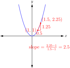
The slope decreased from $3$ to $2.5$ when we made the second point closer to the first, and excitingly, the red line with this slope appears to more closely match the blue curve between those points! Of course, we don’t want to keep doing slope calculations with smaller and smaller decimals to get closer and closer approximations; we want to cut to the chase and take the best possible approximation, which would be the secant line formed by two distinct points as close together as possible.

How can we find the slope of this best possible secant line? By using a limit!

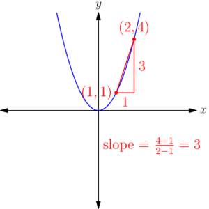
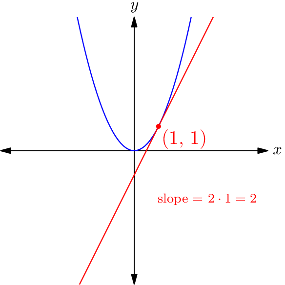
Here’s the idea: we’ll leave our first point $(1,1)$ as-is, and express the second point as being at an $x$-coordinate of $1 + h,$ where $h$ represents the horizontal distance (aka the “run”) between the two points. (In our first slope calculation, we had $h = 1.$ In our second, we had $h = 0.5.)$ The second point must be on the graph of $y = x^2,$ so its $y$-coordinate must be $(1+h)^2.$ Our general slope calculation therefore looks like $$m = \frac{(1 + h)^2 \,-\, 1}{(1 + h) \,- \,1}.$$ Expanding this out and simplifying, we have $$\begin{align*} m &= \frac{1 + 2h + h^2 \,- \,1}{1 + h \,-\, 1} \\ &= \frac{2h + h^2}{h} \\ &= 2 + h \end{align*}$$ for the slope of the line between $(1,1)$ and the point $h$ units to the right of it.

Our best possible secant line has these two points as close together as possible, which means we should look at what happens when $h$ (the distance between them) approaches zero: $$m = \lim_{h\to 0} 2+h = 2.$$

Would you look at that — we just found the slope of $y = x^2$ at $x = 1$! 😄

This example was quite specific, though, so let’s see if we can generalise this process to arbitrary points and arbitrary functions. Suppose we wanted to find the slope of $y = x^2$ at any point, rather than specifically at $(1,1).$ In that case, we could write our first point as $(x, x^2)$ and our second point as $(x + h, (x + h)^2).$ The limit of the slope between these points would then be $$\begin{align*} m &= \lim_{h \to 0} \frac{(x+h)^2 \,-\, x^2}{(x+h) \,-\, x} \\ &= \lim_{h \to 0} \frac{x^2 + 2xh + h^2 — x^2}{h} \\ &= \lim_{h \to 0} 2x + h \\ &= 2x. \end{align*}$$

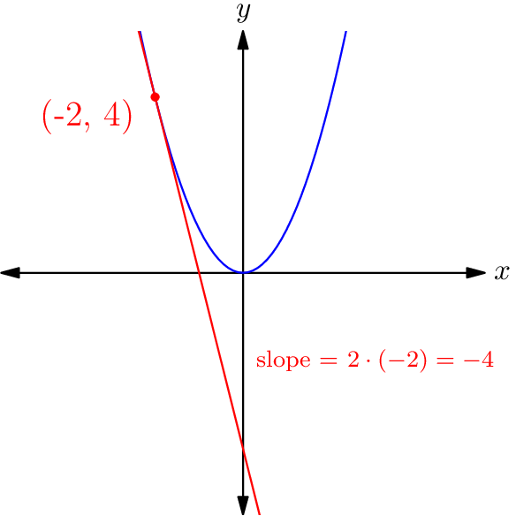
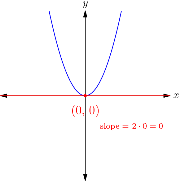
This is our coveted slope-as-a-function-of-$x$! Whatever point we’re looking at on the graph of $y = x^2,$ this tells us that the slope of the graph at that point is simply two times the $x$-coordinate of that point.

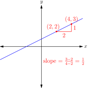
  1. A coordinate pair $(x,y)$ is included in the graph of a function exactly when it satisfies the equation defining the function, so saying that these two points are "on the line" is equivalent to saying that they each satisfy the linear equation.
  2. Note that we get the same value of $m$ if we subtract the second coordinate pair from the first (rather than subtracting the first from the second). The important thing is to use the same order in the numerator as we do in the denominator, whichever order we pick.
  3. As we'll see later on, it turns out that the slope of this secant line is the average slope of the function between those points.